Chapter 2 Methods
All code used in this project can be accessed at https://github.com/aaronsk7/guppy-methylation
2.1 Experimental System
2.1.1 Animal Collection, Care and Treatment
The foundation of the experimental guppy population was extracted from Alligator Creek in Bowling Green Bay National Park where they were introduced 50 to 100 years ago. The light environments which guppies inhabit within this area is varied, however open canopy streams are their most common light environment . Therefore, the ancestral populations of these guppies likely experienced broad-spectrum light conditions (Kranz et al. 2018).
The foundation population consisted of 300 adult fish and 50 juveniles but the effective population size was probably larger as females store sperm, leading to a mean of 3.5 sires per brood in nature (Kranz et al. 2018). This foundation population was separated into 12 tanks of dimensions 3 m × 1.5 m × 0.5 m deep. To accomplish this. The originally extracted fish were propagated in a single tank until >1000 guppies were present and then the population was divided into two more tanks. The population was once again enlarged and then divided into 4 more tanks and so on until 12 tanks were full. This was done to ensure that each tank had similar genetic diversity and to reduce the impact of founder effects and the resulting genetic drift of these founder effects on the different populations (Kranz et al. 2018).
All tanks were maintained in a constant temperature room at 24 ± 1°C and were illuminated from above using four low flicker (200 Hz) daylight fluorescent tubes under a 12:12 hour light-dark cycle. Population density was maintained at ~1000 fish per tank and all fish were fed a combination of brine shrimp nauplii (Artemia salina; INVE Aquaculture Inc.), algae discs (Wardley), and flakes (Fish Breeders Choice) daily (Kranz et al. 2018).
2.1.2 Ambient Light Treatments
The 12 populations were propagated under three different light conditions (4 tanks per light condition). The overhead light was filtered through a “moss green” filter (Roscolux, filter number 89), a “Lilac” filter (Roscolux, filter number 55), or a clear film filter (functioning as a neutral density filter control to equalize total irradiance with the two other treatments without changing the lab light spectrum). This resulted in 3 treatment groups labeled Green-F89, Lilac-F55, and Clear-CF. Green-F89 was similar to forest shade natural light environments and Lilac-F55 and Clear-CF were more similar to small gap natural light environments. Each light environment differentially stimulated guppy cones types (Kranz et al. 2018).
2.2 Sample preparation
| Kit | Tank 9 (green) | Tank 11 (clear) | Tank 12 (lilac) |
|---|---|---|---|
| New kit | T11-F-N | T11-F-N | T12-F-N |
| Old kit | T11-F-N | T11-F-N | T12-F-N |
A pilot study was performed to determine the reliability of the NEBNext® Enzymatic Methyl-sequencing kit. Using the kit, methylation profiling was performed on 3 individual guppies at the Deakin Genomics Centre, Waurn Ponds. These guppies were extracted from 3 different tanks, each containing a different light condition population. The sequencing of the guppies was performed twice. The first sequencing procedure had older controls spiked-in (from an expired kit stored in the Deakin Genomics Centre) and the other was sequenced with newer controls spiked-in.
The same DNA extraction procedure was followed for both the pilot and main study. In the main study, DNA was extracted from 20 fish per light condition population and 60 fish from the foundation population were thawed out for DNA extraction. Fish were obtained from three populations (replicates) per light condition. DNA was extracted from the eye and brain tissue of the fish. The tissue was cut into small pieces and placed into a 380 µL lysis buffer (50 mM Tris-HCl, 10 mM EDTA, 20% SDS) and 20 µL Proteinase K (>600mAU/mL) to be digested overnight. Protein precipitation was performed by adding 100 µL saturated > 5M KCl to the samples which were then incubated on ice. 1x volume of chloroform was added to them before the aqueous layer of the samples containing the DNA was transferred into a new tube. DNA was precipitated using 1x volume of isopropanol and was then washed using 1mL 80% ethanol. The DNA was then eluted in 100 µL of elution buffer (10 mM Tris-HCl, 1 mM EDTA). The DNA extracted from each fish was combined according to the population from which the fish was obtained
The genomic DNA of the samples was quantified with High-sensitivity assays (Invitrogen, USA) using a Qubit 4.0 Fluorometer (Invitrogen, USA). The quality of the DNA was accessed on 4200 TapeStation System (Agilent, USA) and Nanodrop 2000 (Thermofisher, USA).
The pUC19 plasmid DNA and Lambda phage DNA were spiked into each of the sequencing samples in order to act as controls and to therefore better gage the reliability of the kit. The pUC19 plasmid DNA and the Lambda phage DNA came with the NEBNext® EM-seq kit. For each sample, the controls were diluted to a 1:100 ratio before 2 µL of the diluted solution were added to 200 ng of genomic DNA (in a volume of 50 µL). The DNA was sonicated to a target size of 240-290 bp using a Q800R sonicator (Qsonica, USA). The parameters used were: 20% amplitude, pulse on 15 seconds, pulse off 15 seconds, temperature 4°C for 10 minutes. The sonicated DNA was prepped using the NEBnext® Enzymatic Methyl-seq Kit (New England Biolabs, Ipswich, MA) in line with the manufacturer’s protocol. The PCR enrichment of adaptor-ligated DNA was repeated for a total of 5 cycles. Sodium hydroxide was used for the denaturation step of the PCR. Quantification and size estimation of the libraries was performed on both the Qubit 4.0 Fluorometer and 4200 TapeStation System (Agilent, USA).
For the main study 2 µL of each library were pooled into a new microfuge tube and enzymatically treated with Illumina Free Adapter Blocking Reagent (Illumina, USA). The pooled library was pre-sequenced on the MiniSeq Sequencer (2 x 150 bp paired-end reads) (Illumina, San Diego, USA) to obtain the read distribution of each sample. Each library was then re-pooled to equal molar concentrations, enzymatic treated, denatured and normalized to 2 nM. Finally, the library was sequenced on the NovaSeq 6000 Sequencer (2 x 150 bp paired-end reads) (Illumina, San Diego, USA) at the Deakin University Genomics Centre. While the same process was followed for the pilot study, Only the MiniSeq sequencing system was used.
2.3 Data Processing (section 2.3)
After the sequencing was performed the read data was loaded onto a computer and this data was run through a data processing pipeline. The first step of this pipeline involved using the software Skewer v0.2.2 (Jiang et al. 2014). This software is used to trim the adapters from the paired end reads. Skewer also trims reads based on a threshold quality score which measures the likelihood of an individual base being called correctly. This threshold was set to a quality score of 20 to remove bases with poor quality from the 3’ end.
To determine the genomic origin order of the trimmed reads, Biscuit v0.3.16.20200420 was used to map reads to the Poecilia reticulata reference genome. The reference genome was downloaded from Ensembl (https://m.ensembl.org/Poecilia_reticulata/Info/Annotation#assembly). SAMblaster v0.1.26 (Faust and Hall 2014) then removed duplicate reads from the SAM file generated by Biscuit and SAMtools v1.12 sorted the mapped SAM/BAM file by genomic location. Lastly MultiQC (Ewels et al. 2016) v1.9 compiled quality metrics from the bioinformatics analyses performed. From this, a single report detailing the results of each analysis was generated.
2.4 Pilot Study/Main QC Charts (section 2.4)
Using the data derived from the pilot and main study a series of charts were created using R studio v1.4.1106. The code used to create the pilot study charts can be accessed at https://github.com/aaronsk7/guppy-methylation/blob/main/test_data2/methqc.Rmd and the code used to create the main study charts can be accessed at https://github.com/aaronsk7/guppy-methylation/blob/main/methmaindata.Rmd. The methylation data has been deposited in the SRA (sequence read archive).
2.4.1 FastQC Charts - Unique, Duplicate, Total Reads, GC Content and Trimmed (section 2.5)
FastQC v0.11.9 was used to generate the number of unique, duplicate and total reads in each sample. This data was loaded into R studio and values were generated using base R v4.1.0 functions. Three charts were created in R studio using this data.
FastQC was also used to extract the percentage of reads trimmed by skewer as well as the percentage of GC content within each sample. This data was also loaded into R studio and values were generated using base R functions. A chart depicting GC content data was created using R studio.
2.4.2 Read Length (section 2.5.1)
A shell script was created to count the average read length after trimming from each sample. This data was loaded into R studio and a chart displaying the average read length was created using base R functions.
2.4.3 Insert Length (section 2.5.2)
Using a shell script, the insert lengths of each sample were extracted from the BAM files produced by biscuit using the bamtobed utility from Bedtools v2.30.0 (Quinlan and Hall 2010) and then loaded into R studio. To visualise the distribution, a violin plot was created from this data using the vioplot v0.3.6 package in R.
2.4.4 Methylation (section 2.5.3)
Values for CpG, CpHpG, CpHpH, and CpH methylation were extracted from diagnostic files produced by biscuit. These files were loaded into RStudio and our values were generated using base R functions. From these values, a series of bar charts were created.
2.4.5 Wasted Bases (section 2.5.4)
A wasted bases analysis was performed to understand what percentage of originally sequenced bases were actually usable (Percentage yield) and at what stage of the analysis the bases were discarded. A script, which can be accessed at https://github.com/aaronsk7/guppy-methylation/blob/main/test_data2/basecount.sh, extracted the bases available after sequencing (initial number of bases), after trimming, after mapping/removing duplicates and after removing overlapping reads (figure 2). The number of bases present after each of these processes were loaded into R studio and two charts were made from these values using base R functions. A pie chart was created that displayed the percentage of total wasted bases at each data processing step as well as the total yield. The second chart created was a stacked barplot which displayed the percentage of wasted bases at each data processing step as well as the yield for each sample.
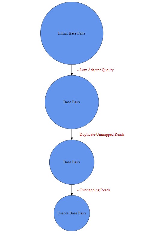
(#fig:figure 2)Illustrates how the useable bases was derived and the order which the bases were removed.
2.4.6 Fold Coverage (section 2.5.5)
For each sample, the amount of usable base pairs (derived from the wasted bases analysis) was divided by the amount of base pairs in the guppy genome to give us the fold coverage for each sample. Using these values, a bar chart was created.
2.5 Principal Component Analysis and Correlation Heatmaps (section 2.6)
The package methylkit was used to perform a PCA analysis at the CpG and region level for all of the light condition samples and the foundation sample. The package gplots was utilised to run a spearman and pearson correlation heatmap. The script to create these plots can be found at https://github.com/aaronsk7/guppy-methylation/blob/main/PCAanalysis.Rmd. Methylation data for each sample was loaded into R and formatted so that it can be handled by methylkit. CpG sites were aggregated within 1000 bp tiles. A PCA analyses and Pearson/Spearman correlation heatmaps were created using both the CpG site and tile data.
2.6 Differential Methylation Analysis (section 2.7)
Differential methylation analysis is used to identify CpG sites or genomic regions which are differentially methylated between experimental/study groups. There are many different bioinformatics software designed for this kind of analysis. The different tools have their own benefits and drawbacks and use different statistical tests to perform the analysis (https://www.ncbi.nlm.nih.gov/pmc/articles/PMC4165320/). For this project we used the packages dmrseq and methylkit.
2.6.1 dmrseq (section 2.7.1)
The bioinformatics software dmrseq was used to perform differential methylation analysis at the region level. The script used to perform this analysis can be found at https://github.com/aaronsk7/guppy-methylation/blob/main/MDDMA.rmd. Methylation data for each sample was loaded into R and formatted to include the information dmrseq requires to perform differential methylation analysis. This included the chromosome and location of each CpG site as well as the coverage and the number of methylated reads at each CpG site. All of the information required to run dmrseq, can be found at the relevant vignette: https://bioconductor.org/packages/release/bioc/vignettes/dmrseq/inst/doc/dmrseq.html.
Differential methylation analysis was performed on each light group comparison (clear versus green, clear versus lilac and green versus lilac) using dmrseq and the output was saved as an rds file for further analysis. Differential methylation analysis was not performed using the foundation population as there existed only one population for this group and dmrseq requires at least one biological replicate.
2.6.2 Methylkit (section 2.7.2)
2.6.2.1 CpG Level
The bioinformatics software methylkit was used to perform differential methylation analysis at the CpG level. The script used to perform this analysis can be found at https://github.com/aaronsk7/guppy-methylation/blob/main/run_methylkit.Rmd. Methylation data for each sample was loaded into R and formatted so that it can be handled by methylkit. Methylkit requires the same information as dmrseq to perform differential methylation analysis (see section 2.x) with the addition of the number of unmethylated reads at each site.
2.6.2.2 Region Level
The genome was divided into tiles 1000 bp in length. The CpG sites that were located within the same tile were aggregated together. The differential methylation analysis was then performed using these tiles. All of the information required to run methylkit, can be found at the relevant vignette: https://bioconductor.org/packages/release/bioc/vignettes/methylKit/inst/doc/methylKit.html. Differential methylation analysis was performed on each light group comparison and the results were saved as rds files for later analysis.
2.7 Differential Methylation Figures (section 2.8)
The results of the differential methylation analysis were loaded into different R markdown files and analysed. These scripts can be found at https://github.com/aaronsk7/guppy-methylation/blob/main/dmrseqResultsAnalysis.Rmd and https://github.com/aaronsk7/guppy-methylation/blob/main/methylkitresultsanalysis.Rmd. The guppy genes and their locations on the genome were downloaded from the ensembl website and loaded into R studio. A script was written to find and create a tss file that contains the promoter regions associated with each of the guppy genes. This script can be found at https://github.com/aaronsk7/guppy-methylation/blob/main/gtf2tss.sh. Using the package GenomicFeatures (found on bioconductor) the CpG sites and regions/tiles for each light condition comparison were annotated to the guppy genes and promoter regions. A series of tables were created which displayed the CpG/tile location and the associated methylation change, p-value, q-value and gene.
The package RCircos was used to create RCircos plots of each light condition comparison for the dmrseq results annotated to genes and the methylkit tile results annotated to promoter regions. The methylation data for each sample was loaded into R studio and violin plots and bar charts displaying percentage methylation for each sample were created for the top 15 most differentiated CpGs and tiles associated with gene promoter regions. Lastly, the genes with the most differentially methylated tiles in their promoter regions were made into a bar graph which displayed the amount of tiles associated with the gene and the direction of the differential methylation (negative/positive). A barplot of this kind was created for each of the light condition comparisons.
2.8 Identified Tiles (section 2.9)
Genes which either possessed tiles in their promoter regions which were associated with low q-values, had multiple significantly differentiated tiles in their promoter regions or were associated with a biological function that could be linked to the experimental conditions were investigated further. For each gene of this kind, a barplot, violin plot and beeswarm plot was created using the percentage of CpG methylation for each sample.
2.9 Enrichment Analysis
A gene set enrichment analysis was performed to identify biological pathways that are significantly enriched between light conditions groups. Two packages, Cluster Profiler and mitch, were harnessed to conduct different types of enrichment analyses. The package mitch was used to perform a functional class sorting enrichment analysis and Cluster Profiler was used to perform an over representation analysis.
The guppy gene ontology data was downloaded from the ensembl website, loaded into R studio and formatted to be handled by both mitch and Cluster Profiler. The methylation tiles located within gene promoters that were identified by methylkit for each light condition comparison were loaded into R studio as well. Using this data, the functional class sorting and over representation enrichment analyses were performed for each light condition comparison.
When performing the over representation analysis, two different analyses were performed for each light condition comparison. In the first analysis, tiles which had a q-value of <0.05 were selected. In the next one, only tiles which had a q-value <0.001 were selected. This was done because such a large number of differentially methylated tiles were obtained and we therefore could afford to select only those which were extremely differentiated and still have a reliable sample size (refer to table x to see the sample size of each comparison). A series of tables containing the results of these analyses were output by mitch and Cluster Profiler.